


Clinical Information Extraction with Large Language Models (LLMs)
Junjing Lin (Takeda), Jianchang Lin (Takeda), Hammaad Adam (MIT), Hillary Keenan (Takeda), Ashia Wilson (MIT), Marzyeh Ghassemi (MIT)


Highlights
While LLMs have been widely hyped as a transformative tool for healthcare, actual applications of LLMs in clinical development remain limited.
Understanding the fundamentals of large language models will help appreciating the challenges and opportunities of using these innovative tools.
Emerging applications of LLMs show promises in changing the way we solve medicine problems.
… In effect, we are in the process of turning medicine into an information technology, harnessing the exponential progress that characterizes these technologies to master the software of biology.
- Ray Kurzweil, The Singularity is Nearer [1]
While LLMs have been widely hyped as transformative tools for healthcare, actual applications of LLM in drug development remain limited. To appreciate the challenges and opportunities of using these tools, a good grasp of the fundamentals seems necessary. Before discussing some promising applications, we would like to introduce large language models.
A Gentle Introduction to Large Language Models (LLMs)
Where does LLM sit within the realm of Artificial Intelligence (AI)? Figure 1 is one way to visualize the LLMs in the Venn diagram of AI. AI is a broad term that includes the theory and development of computer systems performing tasks normally requiring human intelligence, whereas machine learning (ML) focuses on using data and algorithms to enable computers to imitate how humans learn. Deep neural networks (DNN) are a subset of ML that can process more complex patterns (we will talk a bit more about neural networks in later sections). Concisely, generative AI (GenAI) is a type of DNNs that can generate new contents. The process of GenAI learning from existing content is called training and results in a statistical model. When given a prompt, GenAI uses this statistical model to make probability predictions of expected responses; these predicted probabilities will be used to create new contents according to generation rules. Compared to other modality generators, LLM is a type of generative AI that handles text contents.

To apprehend how LLMs come to existence, it may be beneficial to explore the brief history (Figure 2). AI systems were traditionally about perceiving and understanding data rather than on generating them. This distinction marks the main difference between Perceptive and Generative AI, which did not take off until around 2020.
Around 1800s, Legendre and Gauss used linear regression, the simplest kind of forward neural network (FNN), to predict planetary movement. In 1925, Ising model was used to explain why magnets demagnetize when heated sufficiently. This model is considered as the first non-learning recurrent neural network (RNN). Single-layer perceptron was invented in 1957, and can solve binary classification problems that are linearly separable. To overcome the limitation of single-layer perceptron, deep learning network was invented in late 1960s to classify non-linearly separable pattern. In 1972 adaptive RNNs started to emerge; they overcame FNN’s inability to retain previous input by using hidden states to capture sequential dependencies. In late 1990s, long short-term memory (LSTM) networks, as a variation of RNN, improved the ability to handle long-term dependencies by using gated cells in the hidden layers to have better control of information flow and memory manipulations. In 2017, transformer natural language processing (NLP) models were set in motion upon the rise of the transformer architecture. Transformers could generalize better than the then-prevailing RNNs and LSTMs. However, from today’s point of view, models developed during this period had limited capabilities, mainly due to the lack of large datasets and adequate computational resources.
LLM NLP models were popularized by the launch of OpenAI’s GPT-3 in 2020. LLMs like GPT-3 were trained on massive amounts of data, which allowed them to produce more accurate and comprehensive responses compared to previous models. Notably, LLMs made NLP models much more accessible to non-technical users who could now solve a variety of tasks just by using natural-language prompts.

The Architecture of LLM
As mentioned in Figure 1, LLM is a type of neural networks (NN). NNs are machine learning algorithms loosely modeled after the human brain. Like human brain, artificial NNs consist of neurons, aka. nodes, that are responsible for all the model functions. There are usually at least three layers: input layer, passing input data to the rest of the network; hidden layer (s): performing specific functions such as classifying or generating data, etc.; output layer, generating prediction or classification. Next, I will explain how LLM architecture relates to several common NN architectures (Figures 3a-3d).
The first architecture is FNN (Figure 3a). In FNN, the information comes inside the model through the input layer, passes through the series of hidden layers, and finally goes to the output layer. This Neural Networks architecture is forward in nature. The later layers give no feedback to the previous layers. The second architecture is RNN (Figure 3b). In RNN, the input is in the form of sequential data that is fed into the RNN, which has a hidden internal state that gets updated every time it reads the sequence of data in the input. The internal hidden state will be fed back to the model. Such capability of relating to past data make RNN good at many NLP tasks, especially sentiment analysis and text classification. Another architecture is generative adversarial network (GAN) (Figure 3c). GAN is a generative model and is used to generate entirely new synthetic data by learning the pattern. It has two components—a generator and a discriminator that work in a competitive fashion. The generator takes in random data as input and returns generated data. The discriminator acts as a critic and strives to distinguish between samples from the training data (real sample) and samples produced from the generator (faked sample). There is feedback from the discriminator fed to the generator to improve the performance.
GAN is often used for data generation; however, it does not work very well in text generation, due to some inherent challenges in processing texts in this model. While RNNs have their advantages, they can only take data sequentially and are very slow to train; it also cannot process longer data sequences and consider the overall context of the input sequence. Transformer architecture was introduced to solve these limitations ---- it can process all the words in the sequence in parallel while capturing long-range dependencies, thus greatly speeding up computation.
In Figure 3d, the example transformer consists of an encoder layer and a decoder layer. In practice, the encoder or decoder stack can include multiple encoder or decoder layers. Both the encoder and decoder contain a feed-forward layer and a self-attention layer, which computes the relationship between different words in the sequence. The decoder contains a second encoder-decoder attention layer, which produces a representation for each target sequence that captures the influence from the input sequence as well. Attention mechanism is probably the most important feature in transformer architecture. It helps transformer understand the context between words in a sentence, allowing it to focus on the most relevant information. The transformer has two embedding and position encoding layers. The input sequence or target sequence is first fed to the embedding layer. The embedding layer maps each input token (like words or subwords) into a high-dimensional embedding vector, which is a richer representation of the meaning of that word. Then position encodings are added to the embedding to provide information about the position of each token in the sequence, as transformer processes all tokens in a sequence in parallel, losing the position information. When generating output, the decoder FNN layer projects the decoder vector into word scores, with a score value for each unique word in the target vocabulary, at each position in the sentence. The softmax layer then turns those scores into probabilities. In each position, we can find the index for the word with the highest probabilities, for example, then map that index to the corresponding word in the vocabulary. Those words then form the output sequence of the transformer.

In the above illustration, the transformer contains both an encoder and a decoder, but in practice, LLM can utilize one of the three architecture types. The first type is encoder only architecture, or autoencoding transformer. This architecture is bidirectional, meaning that it can understand the meaning of a word by taking into account both the words that come before and after it in a sentence. LLMs with this architecture are often pretrained with masked language modeling, where the model is asked to predict a masked word by using the surrounding words. This helps the model learn the context and relationships between words in a sentence. A typical example in this category is BERT. A second type is decoder only architecture, or autoregressive transformer. This architecture is unidirectional, as decoder constrains the self-attention by masking the tokens to the right. LLMs of this type are often pretrained with causal language modeling, which trains the model to predict the next token in a sequence based on the previous (predicted) tokens. Many of the popular LLMs fall under this category: GPT, Claude, etc. Last but not least, the encoder-decoder, or sequence-to-sequence architecture. LLMs with this type are often pretrained with corrupted spans of texts, making them good at more complex tasks. Some examples include BART, FLAN-T5 and Megatron-LM (Table 1).
Table 1. Transformer Architecture Types of LLM

Different Ways of Adapting LLMs
In general, the foundation models or models pretrained for general purposes do not work very well for very specific tasks or specialty domains. There are different ways to adapt LLMs for specific purposes (Figure 4). One strategy is through prompt engineering. Prompt engineering only requires modifying prompts without touching the model parameters. Some common methods include zero-shot learning which involves giving the AI a task without any prior examples. You describe instructions in detail, assuming the AI has no prior knowledge of the task; one/few-shot learning: you provide one or more examples along with your prompt. This helps the AI understand the context or pattern you’re expecting; chain-of-thought prompting provides the AI to detail its thought process step-by-step. This is particularly useful for complex reasoning tasks; tree-of-thought technique generalizes chain-of-thought prompting. It prompts the model to generate one or more possible next steps. Then it runs the model on each possible next step using a tree search method. There are many other prompting strategies, which will not be exhausted here.
An important strategy to adapt LLM is fine-tuning, which is essentially a supervised learning process where labeled examples are used to update the model parameters of the LLM. Full fine-tuning will result in a new version of the model with updated parameters. Some potential downsides of this method include computing cost and catastrophic forgetting, where LLM forgets how to do old tasks after learning new ones. Possible ways to mitigate this are to fine tune multiple tasks at one time, or to perform parameter efficient fine-tuning (PEFT).
PEFT is a set of techniques that preserves the parameters of the original LLM and trains only a small number of task-specific adapter layers and parameters. Selective methods are those that fine-tune only a subset of the original LLM parameters. Reparameterization methods also work with the original LLM parameters but reduce the number of parameters to train by creating new low rank transformations of the original network parameters. Lastly, additive methods carry out fine-tuning by keeping all the original LLM parameters frozen and introducing new trainable components.

Another common strategy to adapt LLM is reinforcement learning from human feedback (RLHF). First, you'll pass a prompt from your prompt dataset. Next, you send the completion from the initial LLM, and the original prompt as the prompt completion pair to the reward model. The reward model evaluates the pair based on the human feedback it was trained on and returns a reward value. You'll then pass this reward value for the prompt completion pair to the reinforcement learning algorithm to update the parameters of the LLM, and move it towards generating more aligned, higher reward responses. If the process is working well, you'll see the reward improving after each iteration as the model generates text that is increasingly aligned with human preferences. You will continue this iterative process until your model is aligned based on some evaluation criteria.
Understanding the Size of LLMs
The sizes of LLMs are close to mystical, because they are often too large to be comprehended. However, the sizes of LLM impact practical decision making when we apply LLMs in a resource-constrained world. In general, using larger LLMs that are trained on bigger datasets may have better performance, but they may be too costly in terms of time, computing resources, and even negative environmental impact (depending on energy sources, training time, hardware).
One common aspect to see the size of LLMs is the number of model parameters. Model parameters can be considered as adjustable “dials” associated with the individual neurons in the neural network models. As the training process proceeds, these parameters get updated to optimize the model’s performance on a specific task. To visualize this, if we imagine one parameter takes a space 1cm x 1cm then GPT-2 takes up about 20 soccer fields whereas GPT-4 takes up about 30000 soccer fields (a soccer field =around 60 million parameters). Another aspect of LLM size is training data size in terms of number of tokens. A token can be a word, sub-word or character, depending on how the training text is divided into tokens. Note that most recent LLM only need single pass of the entire training dataset. Let’s imagine one book contains 100,000 tokens, a library shelf holding 100 books (each shelf holds about 10 million tokens), with 0.5 meters per shelf, then GPT-2 is about 1.4 km of shelves whereas GPT-4 is about 650 km of shelves. A third aspect of LLM size is the total number of computations required for training or inference, in terms of GFLOPS. FLOPS stands for floating-point operations ---- a computer doing one addition or subtraction can be considered as one FLOP. GFLOPS is 1 billion FLOPs. An average modern laptop compute about 100 GFLOPs per second at FP32 precision, the GPT-2 will take about 1600 years to be trained on an average laptop, whereas GPT-4 will take about 7 million years! Training is such a tremendous effort, but how about inference using a pretrained model? To understand how training and inference time can be different, here are rules of thumb: #. training computations = 6 x #. parameters x #. tokens; #. inference computations = 2 x #. parameters x input and output length (tokens).

Applications of LLM in Information Extraction
Recent work has demonstrated that LLMs are powerful tools for information extraction, especially tasks such as literature review [3,4,5,6]. In an MIT-Takeda collaboration project [7], we investigated organ transplantation decision process using real-world data (RWD) from electronic health records. However, like many routine care clinical databases, many critical variables, such as lab results, are inconsistently noted in structured fields and are commonly found in free-text case notes. The data we have is a large corpus of 43,819 notes on 14,442 potential donors. These notes contained detailed information on the potential donor’s hospital admission, diagnostic tests, brain death testing, and family interactions. We focus on 8 numeric variables: BUN, creatinine, AST, ALT, Tbili, systolic blood pressure, diastolic blood pressure, and heart rate. Of note, BUN and creatinine are measures of kidney function; AST, ALT, and Tbili are measures of liver function. These values are captured extremely inconsistently in the case notes. For example, many different abbreviations are used for creatinine: “crea”, “cr”, “creat”, and “creatine”; different measurements are also listed in different ways like the example in Figure 6, e.g., measurements of BUN and creatinine may be listed sequentially or together.
The highlighted texts in Figure 6 are an example of inconsistent lab result presentation containing similar information: on the left, each test code is followed by numeric result, separated by space, grouped by comma; on the right, test codes and results of blood urea nitrogen (BUN) and creatinine (CREA) are concatenated by forward slash, with test code group and result group separated by space; and the test code and result of AST (aspartate aminotransferase) are separate by a colon. This is a relatively easy task for human to distinguish, but it could be challenging to ask computer to extract relevant information, using standard extraction technique, such as regular expression. The question is: can we use LLM to extract numeric info from unstructured texts?

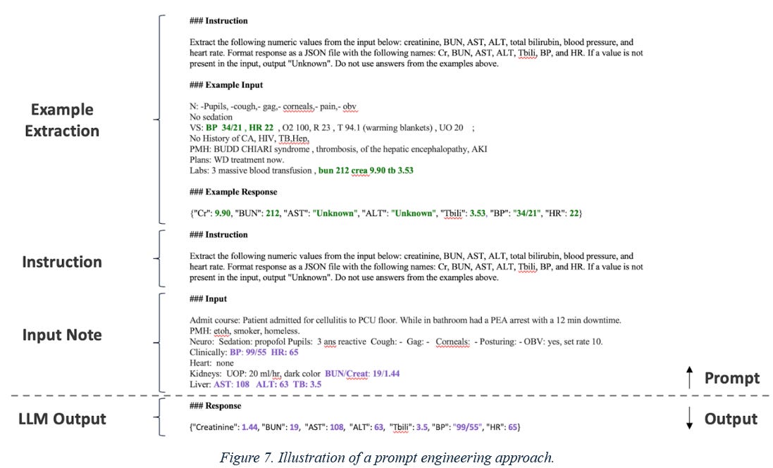
As mentioned in previous sections, foundation LLMs are often not pretrained to be efficient in specialty domains, such as medicine. And LLM model fine-tuning for specific tasks are generally challenging due to limited computing resources/infrastructure. Based on these considerations, we proposed a prompting engineering strategy for numeric extraction from unstructured clinical notes and novel heuristics to combat hallucination. This approach provides LLM with a tailored prompt that primed it to generate text summarizing the eight clinical variables contained in a given free-text note. It is an application of in-context learning, where an LLM can learn to perform a task by analogy (i.e., from an example provided in the prompt) instead of further training on labeled data. While the prompt in Figure 7 provides only one example to the LLM, we considered approaches that provide more examples (or “shots”) in our experiments. We varied the number of examples provided between one (i.e., “one-shot”) and five (“five-shot”).
Our approach used the Llama-2 model, an open-source pre-trained LLM from Meta. We chose “Chat-HF” version of Llama-2 as this version is specifically trained to generate text that conforms to user-specified instructions, thus being the best fit for our extraction task. In addition, we picked the smallest version of Llama-2 (i.e., Llama-2 7B) because it fits on a single GPU with under 25GB of RAM when loaded in half-precision floating point format. As you can see, this choice was dictated by computational constraints: the PHI-compliant server on which the notes were stored did not have sufficient RAM to host larger models. Using larger models would likely have provided better results; however, our work demonstrates that our approach can be effective even in settings with computational constraints.
A frequently observed problem with LLMs is their tendency to “hallucinate,” that is, generate plausible but incorrect information. Our LLM approach occasionally exhibited such behavior; for example, the LLM sometimes outputs a common value of 1.5 for creatinine, even if no mention of creatinine was made in the note. So we implemented three heuristics that detected hallucinations and increased the accuracy of our LLM extractions. The first heuristic is to cross-check original note. For example, if the LLM extracted a BUN value of 16, we checked if the number 16 was present in the original text. If it was not, we replaced the extracted value with null. The second heuristic 2 is to remove values from examples in the prompt. We observed a tendency for the LLM to output values from the examples in the prompt if no value was specified in the input note. We thus introduced a second heuristic which replaced extracted values with nulls if they were present in one of the five example notes. For example, suppose the example provided to the LLM had a BUN value of 212. Thus, if the LLM predicted a BUN of 212 for the target note, we replaced it with null. The third heuristic is to remove any extracted values that fell outside plausible ranges for the corresponding variables. For example, a creatinine value of 30 is extremely rare and can likely be discarded as an inaccurate extraction.
To evaluate the model performance, we consider three performance metrics: accuracy, precision and recall. We used an annotated subset of 298 notes to evaluate the performance of our LLM approach. These notes were hand-annotated, and manually inspected to extract the values of the eight relevant variables. The annotated notes were randomly-selected from the overall corpus and were randomly split into a validation set and a testing set. The baseline comparison is by using a rules-based approach with regular expression.
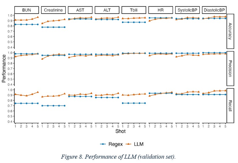
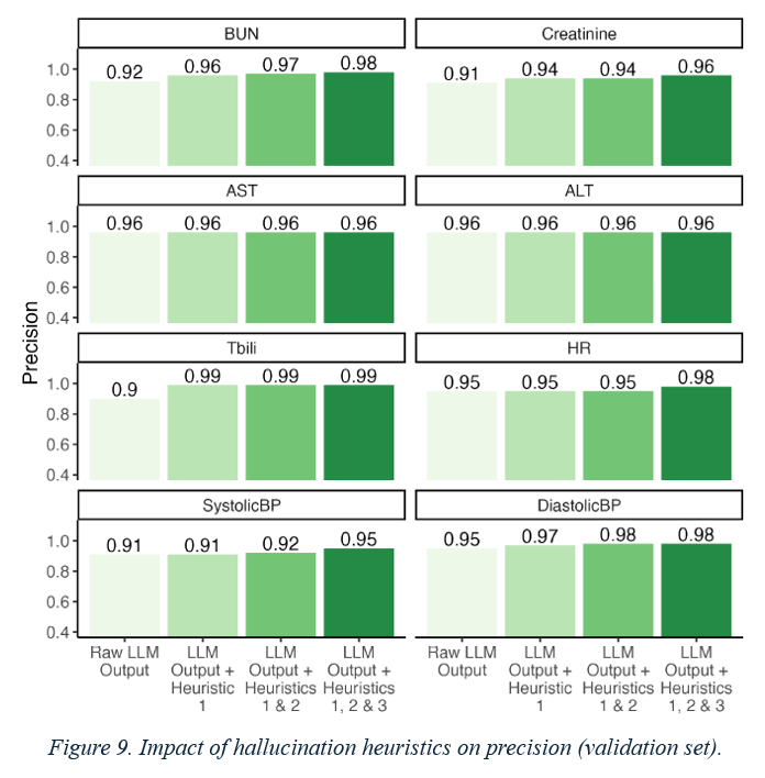
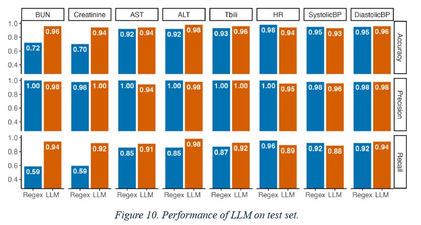
Figure 8 describe the performance of our LLM extraction approach on the validation set. Each row displays a different performance metric (accuracy, precision, and recall) while each column displays a different clinical variable (e.g., BUN, creatinine, etc.). We plot each performance metric as a function of the number of extraction examples provided in the prompt to the LLM (x-axis). The LLM (represented by orange lines) outperforms the regex baseline (represented by blue lines) on both accuracy and recall, while maintaining a similar level of precision. All performance metrics increase with the number of provided examples: the five-shot approach has the highest accuracy, precision, and recall for all variables. Figure 9 shows the impact of the hallucination heuristics on precision in the validation set. Each bar shows the marginal contribution of each heuristic to the precision of the five-shot LLM approach. The hallucination heuristics increased the precision of the LLM approach. While the raw five-shot LLM output has greater than 90% precision for all variables, the hallucination heuristics were able to increase this precision to over 95%. Figure 10 displays the performance of our LLM extraction approach on the test set. Each row displays a different performance metric (accuracy, precision, recall) while each column displays a different numeric variable (e.g., BUN, creatinine, etc.). The LLM (orange) outperformed the regex baseline (blue) on both accuracy and recall, while maintaining a similar level of precision.
One can also consider the value of using LLM on the downstream data analysis. In this case study, LLM extraction greatly increased the completeness of the data. Table 2 summarizes the number of potential donors who had at least one observation of each variable using 1) the tabular data only, 2) the tabular data with regex extractions, and 3) the tabular data with LLM extractions. The LLM extractions greatly improved data completeness; for example, using LLM extractions to supplement the tabular data provided creatinine measurements for an additional 8,064 potential donors (compared to 5,788 additions for the regex approach). Further, this additional data had a direct impact on the data analysis task. Table 3 displays the estimated regression coefficients for BUN, creatinine, AST, and Tbili on the outcome of the organ procurement organization approaching a potential donor’s family. Compared to using tabular data only, using tabular data + LLM enables the identification of four significant variables, which align with clinical expectations. It shows that LLM can increase estimation precision by reducing missing data.

Discussion
Our work provides a practical application for LLMs that can be combined with existing informatics methods to improve real-world data quality in impactful domains. Novel approaches of using LLM can be highly valuable tools, as critical decision making in areas of unmet medical needs increasingly rely on real-world data. We are optimistic that by leveraging innovative tools like LLMs, we can revolutionize the way we address complex medical challenges, much like how we approach technical problems.
Reference
1. Kurzweil, R. (2024). The Singularity Is Nearer: When We Merge with AI. Random House.
2. Stigler, S. M. (1990). The history of statistics: The measurement of uncertainty before 1900. Harvard University Press.
3. Agrawal M, Hegselmann S, et al. Large language models are few-shot clinical information extractors. In: Goldberg Y, Kozareva Z, Zhang Y, editors. Proceedings of the 2022 Conference on Empirical Methods in Natural Language Processing.
4. Dagdelen, J., Dunn A., et al. (2024). Structured information extraction from scientific text with large language models. Nature Communications, 15(1), 1418.
5. Gartlehner, G., Kahwati L., et al. (2024). Data extraction for evidence synthesis using a large language model: A proof‐of‐concept study. Research Synthesis Methods.
6. Khraisha, Q., Put S., et al. (2024). Can large language models replace humans in systematic reviews? Evaluating GPT‐4's efficacy in screening and extracting data from peer‐reviewed and grey literature in multiple languages. Research Synthesis Methods.
7. Adam H., Lin J., et al (2024). Clinical Information Extraction with Large Language Models: A Case Study on Organ Procurement. Proceedings of American Medical Informatics Association Annual Symposium 2024.